• 3-minute read
• 29th November 2020

Microsoft Excel: How to Highlight Cells with Conditional Formatting

Conditional formatting can make the data in a spreadsheet easier to read. One way it can do this is by applying a specific color or style to highlight cells based on their value. But how does it work? In this post, we look at how to highlight cells via the conditional formatting in Microsoft Excel.

How to Highlight Cells with Conditional Formatting

In Microsoft Excel, you can apply styles to cells depending on their content by setting a conditional formatting rule (i.e., a set of conditions in which the formatting will apply). Excel comes with a few pre-set options for this, all of which are available via the Conditional Formatting option on the Home tab.

However, we’re focusing on highlighting cells in this post. To do this:

1. Select the cells you wish to format.
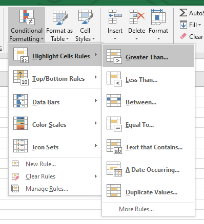
2. Go to Home > Styles > Conditional Formatting on the ribbon.
3. In the drop-down menu, hover the cursor over Highlight Cells Rules.
4. Pick an option from the menu.

This opens a pop-up where you can set a value (i.e., the value or text that triggers the formatting in the selected cell[s]) and a style (i.e., the formatting to apply).

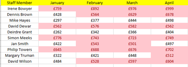
When you’re done, click OK to apply the formatting to your chosen cells. In the example below, we’ve highlighted cells with a value greater than £500.

There are a few options available here, though, so let’s look at them next.

Pre-Set Rules Available in Excel

If you follow the instructions above, you’ll see a list of pre-set rules you can use to highlight cells using conditional formatting:

• Greater Than – Applies the chosen formatting when a cell exceeds the stated value (e.g., in our example above, we’ve set it to apply red shading and text in any cell with a value over 500).
• Less Than – As above but for cells beneath the stated value.
• Between – Applies formatting when a cell falls between two values.
• Equal To – Applies formatting for cells containing an exact value.
• Text that Contains – Formats cells that contain a set word or phrase.
• A Date Occurring – Highlights cells that fall within the set date criteria (e.g., this week, next week, this month, next month).
• Duplicate Values – Highlights cells that contain the same value or text as another cell with the same conditional formatting.

You can also select More Rules from the menu to create a custom formatting a rule. However, the pre-set options should cover most of your basic requirements for highlighting cells based on their values.

Removing Conditional Formatting

Finally, there will be times you wish to remove some or all the conditional formatting rules from your data. This is easy to do:

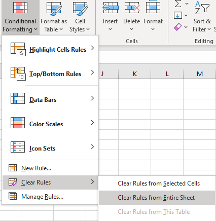
1. Select the cells from which you want to remove formatting.
2. Once again, go to Home > Styles > Conditional Formatting.
3. In the menu, select Clear Rules and click Clear Rules from Selected Cells.

This will remove the formatting as selected. In addition, selecting Manage Rules in the menu will open a list of all the conditional formatting in a spreadsheet. You can then delete or edit rules as required.

Expert Spreadsheet Proofreading

As well as using conditional formatting effectively, you’ll want the text in your spreadsheets to be free from errors. And the best way to do this is to use our spreadsheet proofreading services. We have experts ready to help!